Description: trial-gnuplot.JPG
|
| From: | David M. Cook |
| Subject: | Problem exploiting interpreter property |
| Date: | Fri, 3 Mar 2017 20:50:50 +0000 |
|
3 March 2017 Hello, I am apparently overlooking something in my attempt with OCTAVE 4.0.0 running on a Windows 7 HP laptop to produce an output EPS file of a graph containing labels with some characters modified with TeX-style adjustments, i.e., exploiting
the interpreter property (for which ‘tex’ appears to be the default setting, though adding the option ‘interpreter’, ‘tex’ in the title, xlabel, and ylabel statements below appears to make no difference). Because of the statement “Note that for on-screen display the interpreter property is honored by all graphics toolkits. However for printing,
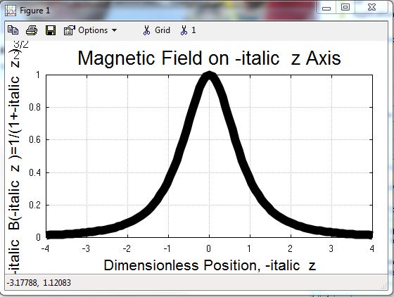
only the in the on-line OCTAVE help at the link https://www.gnu.org/software/octave/doc/v4.0.0/Use-of-the-interpreter-Property.html I use the gnuplot graphics toolkit. The code close all dz = 8.0/100.0; z = [ -4.0 : dz : 4.0 ]; B = (1.0 + z.^2).^(-1.5); graphics_toolkit( ‘gnuplot’ ) plot( z, B, 'color', 'black', 'linewidth', 4 ) grid on title('Magnetic Field on {\it z} Axis', 'FontSize', 20 ) xlabel('Dimensionless Position, {\it z}', 'FontSize', 16 ) ylabel( '{\it B}({\it z} )=1/(1+{\it z}^2)^{3/2}', 'FontSize', 16 ) produces the on-screen graph in the attached file trial-gnuplot.JPG obtained via screencopy. In particular (and contrary to what I expected from the above quotation from the OCTAVE manual), the TeX stipulations \it are not rendered and
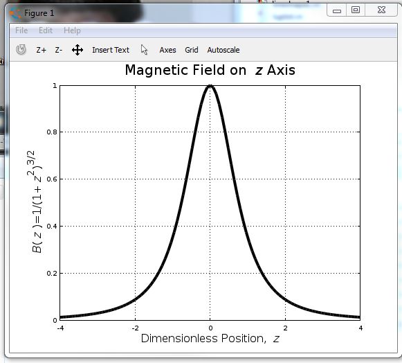
the exponents 2 and 3/2 in the y label are displayed in the wrong orientation. Further, creating an EPS file of this display with the statement print –depsc2 ‘trial-gnuplot.eps’ produces the attached file, which is still not correct. The exponents are properly oriented but the italic specification is rendered differently than in the file trial-gnuplot.JPG. If, however, I continue by executing the code close all graphics_toolkit( ‘qt’ ) plot( z, B, 'color', 'black', 'linewidth', 4 ) grid on title('Magnetic Field on {\it z} Axis', 'FontSize', 20 ) xlabel('Dimensionless Position, {\it z}', 'FontSize', 16 ) ylabel( '{\it B}({\it z} )=1/(1+{\it z}^2)^{3/2}', 'FontSize', 16 ) the resulting on-screen graph, shown in the attached screencopy file trial-qt.JPG, is what I expected and is correct. The EPS file created with the statement print –depsc2 ‘trial-qt.eps’ in the attached file trial-qt.eps does not reflect my intent, indeed, is the same as trial-gnuplot.eps. Based on the above quotation I expected ·
trial-gnuplot.JPG and trial-qt.jpg to be correct. ·
trial-qt.eps to be incorrect. ·
trial-gnuplot.eps to be correct. Note, incidentally, that it seems to be particularly \it that is not properly rendered either on the screen or in the file by gnuplot. If with graphics toolkit gnuplot the y label were, for example, ylabel( ‘\Gamma = 1/(1+\alpha^2)^{3/2}’, ‘FontSize’, 16 ) \Gamma and \alpha would be properly rendered on screen but the exponents would still be incorrectly oriented but the y-axis label in the EPS file produced by the print command would be exactly correct. What am I overlooking or how am I misinterpreting the quotation from the OCTAVE manual? Thanks for your help. David David M. Cook VOICE: 920-832-6721 Department of Physics FAX: 920-832-6962 Lawrence University Email: address@hidden 711 E Boldt Way, SPC24 Appleton, WI 54911 |
![]() trial-gnuplot.JPG
trial-gnuplot.JPG
Description: trial-gnuplot.JPG
![]() trial-gnuplot.eps
trial-gnuplot.eps
Description: trial-gnuplot.eps
![]() trial-qt.JPG
trial-qt.JPG
Description: trial-qt.JPG
![]() trial-qt.eps
trial-qt.eps
Description: trial-qt.eps
| [Prev in Thread] | Current Thread | [Next in Thread] |